Pivot tables are mainly used for a quick summarization and analysis of large amounts of data in lists and tables. Pivot tables are mostly used in excel applications with excel functionalities such as the drill down functionality into raw data. Data in a pivot table are organized in a tabular layout. Each column will have a unique name on every single row, every field will have a value in every single row, and columns will not have repeated groups of data.
Creating a Pivot
Creating a pivot can be done in the newly created report. When the user clicks on the pivots button, a new tab with the default pivot name 'New Pivot1' will be displayed. That particular tab name can be edited either by double clicking or right clicking to change the tab name.
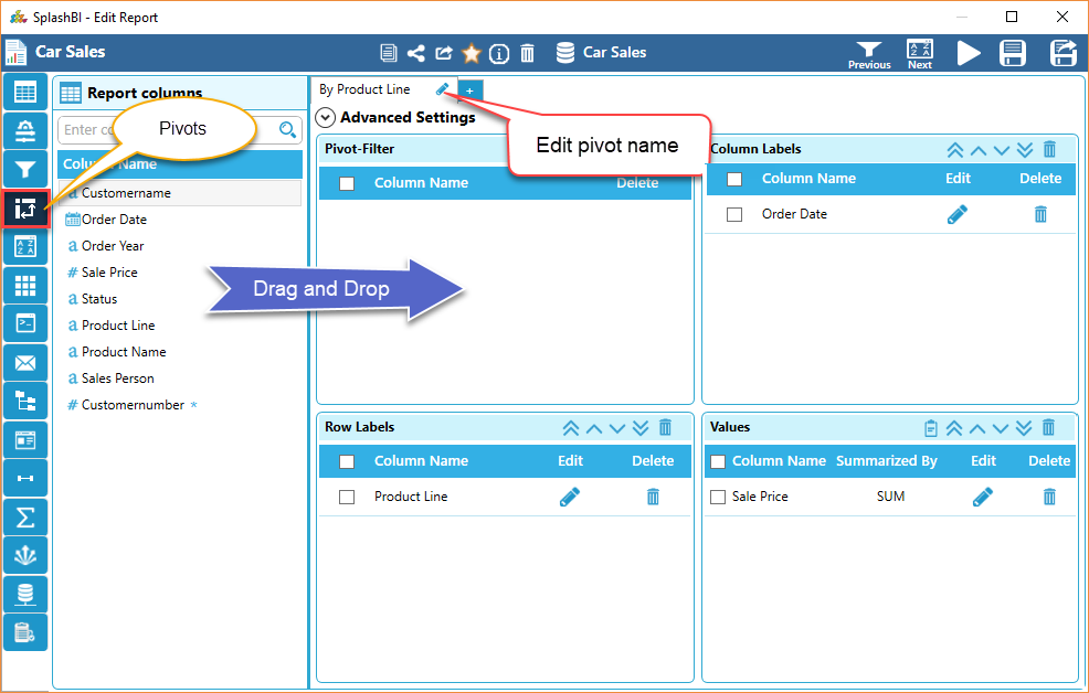
The user can create multiple pivots for the report by clicking the 'Plus' sign ![]() icon. Each and every tab has four small sections. They are Pivot Filters, Column Labels, Row Labels and Values.
icon. Each and every tab has four small sections. They are Pivot Filters, Column Labels, Row Labels and Values.
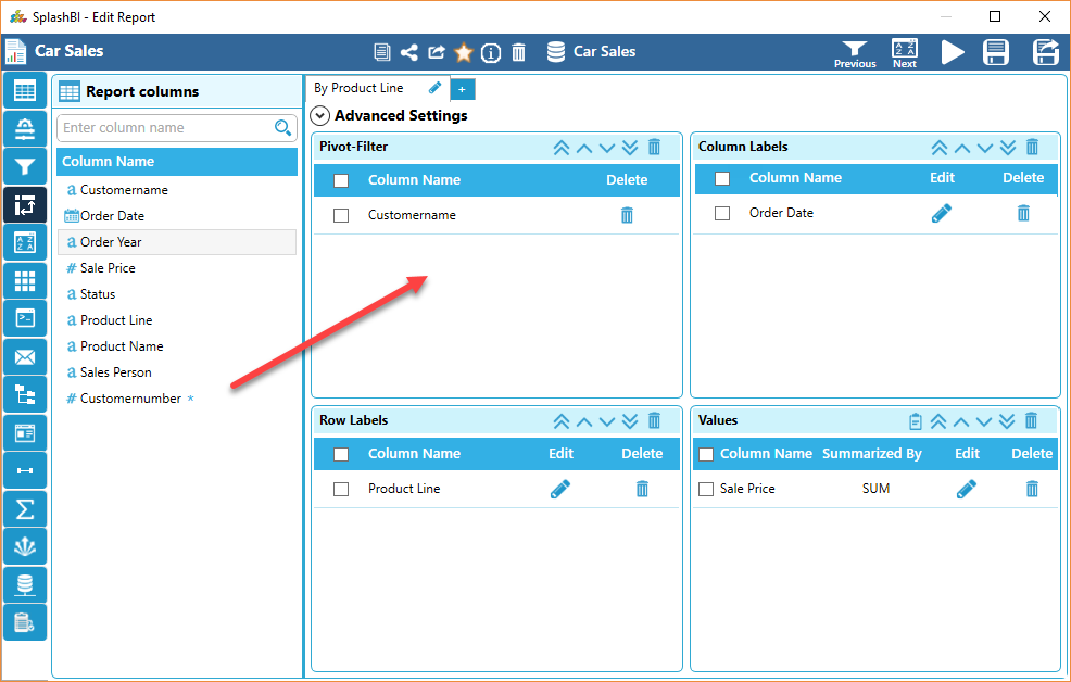
The user can drag and drop report columns from the left side over to the above sections to create a pivot.
The user can delete the pivot tab by clicking on the 'Delete'  icon which will be displayed beside the pivot name. The user can also reorder the values in all sections by using the 'Reorder'
  buttons presented in each section.
° In the Columns section, the user can edit the column to set subtotals by clicking the 'Edit'  Icon.
Icon.
• A pop up window will appear with the Source Column and Sub Total labels.
• To change the sub totals from automatic to another method, click the down arrow .
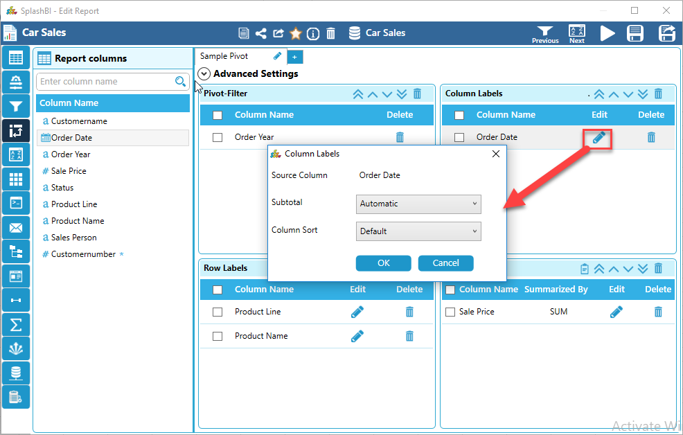
• Click the desired method and click the 'OK' button.
• To exit the edit mode without make a change, click the 'Cancel' button.
° In the Rows section, the user can edit the column to set subtotals by clicking the 'Edit' Icon.
• A pop up window will appear with the Source Column and Sub Total labels.
• To change the sub totals from automatic to another method, click the down arrow  .
.
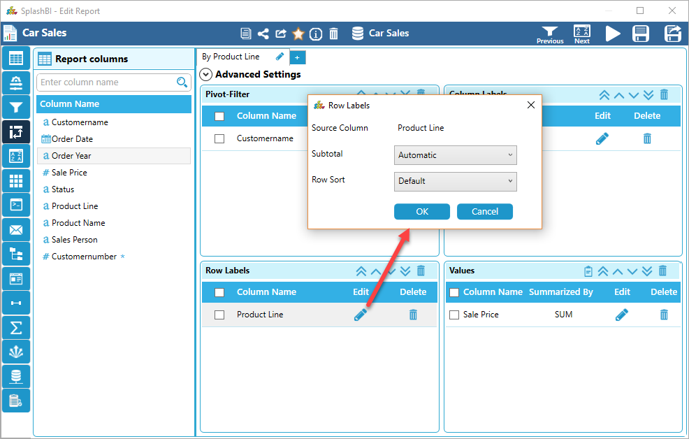
• Click the desired method and click the 'OK' button.
• To exit the edit mode without make a change, click the 'Cancel' button.
In the Values section, the user can edit the column to set Summarized By, Pivot Display Name, and Data Filed Value AS by clicking the 'Edit'  icon.
icon.
• Once the edit icon has been clicked, a pop up window will be displayed.
° To change Summarized By, click the down arrow  to display a list to choose from.
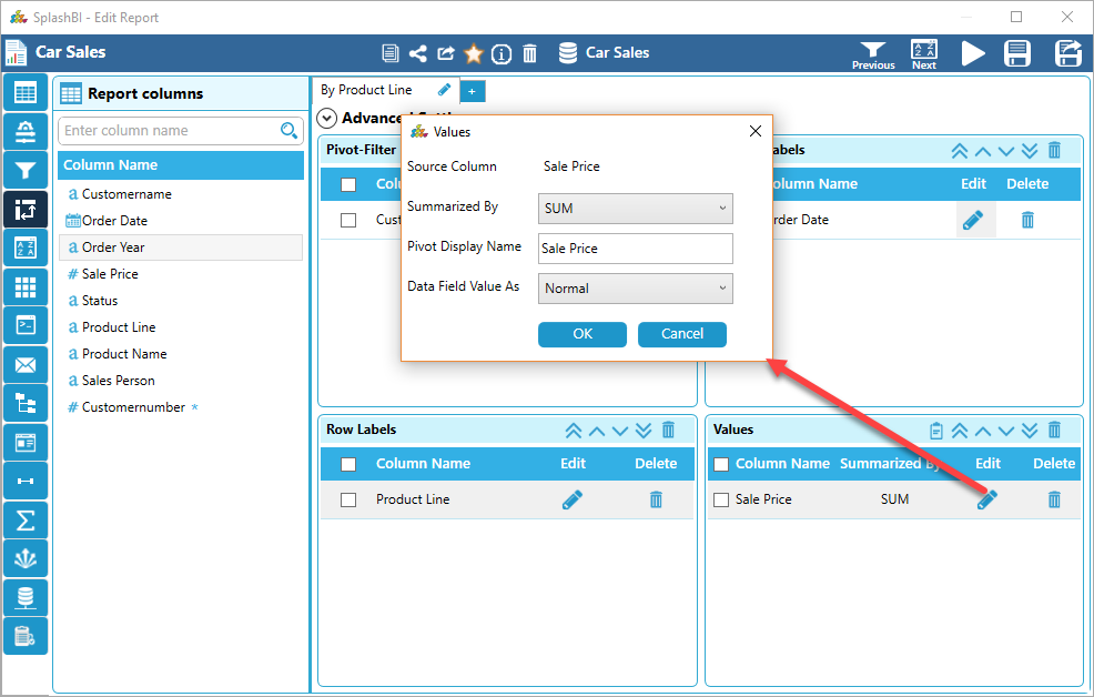
•The display name of the column on pivot can be changed by overwriting the current name in the field.
•To change the Data Value "AS" click the down arrow. There are 3 choices: "Normal", "% of", "% of Row".
°Click the desired method.
•To save changes, click the 'OK' button.
•To exit out of edit mode without saving changes, click the 'Cancel' button.
Summary Calculation Columns:
Add an additional calculation to the columns mentioned in the Values Panel of the Pivot section. The calculated values are available as a part of Excel output.
Drag and drop the column in the values section.
Click the
'Add Summary Calculation Column' ![]() icon to open the summary calculations window. Click the
fx button to enter the calculation column.
icon to open the summary calculations window. Click the
fx button to enter the calculation column.
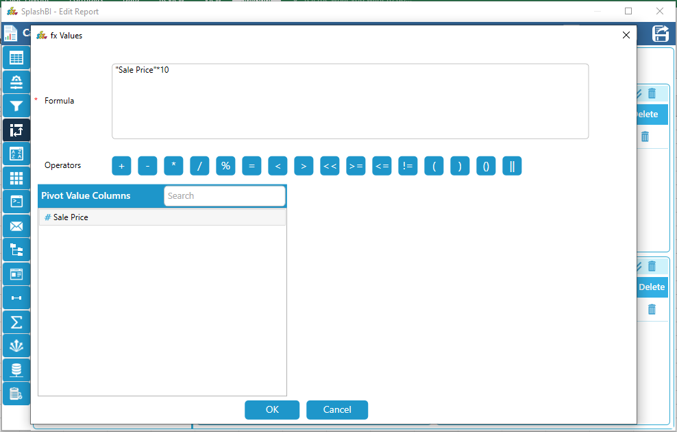
Drag the column and create the formula and click Save.
Fill the other-self explanatory options and click Save.
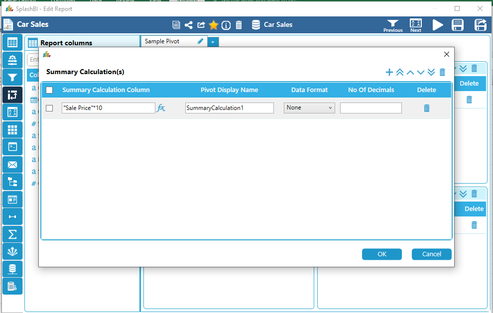
In Excel output, click the Pivot tab to view the output.
Single Level Delete:
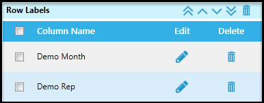
The user can delete single or multiple columns added in all sections by using column level delete, or mass delete icons.
From each section, the user can delete a column one at a time by clicking the 'Delete' ![]() icon from a specific section.
icon from a specific section.
Mass Delete:
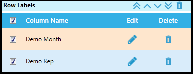
SplashBI Excel Connect allows users to do mass delete columns from each section by clicking the header check box  from a specific section.
• Clicking the check box from the top level of each section will automatically enter check marks for all columns.
• From the tool bar of each section is a 'Delete'  icon, click the delete icon to remove desired
columns from the pivot table.
Advanced Settings:
SplashBI Excel Connect allows the user the ability to change advanced settings of a pivot by clicking on the 'Advanced Settings' 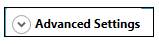 icon at the end of pivot tab, it expands the screen with pivot advanced settings details.
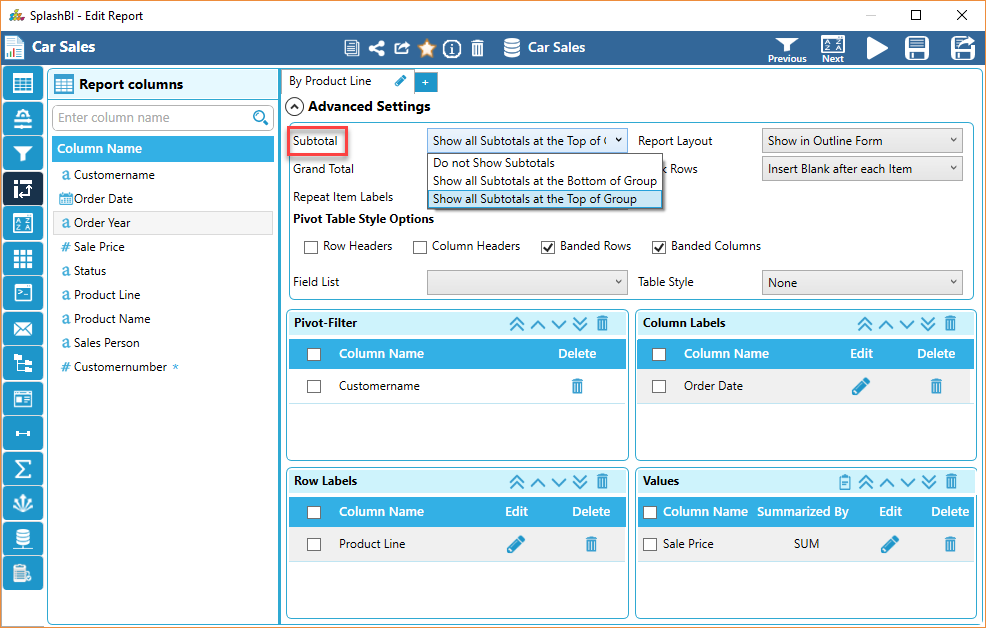
•Once Advanced Settings is clicked, the screen will expand appear to further customize the pivot table.
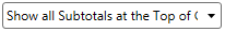
•Sub Totals can be changed to view at the top of the group, bottom of the group, or no sub totals , click the down arrow to display choices and choose by clicking desired method.
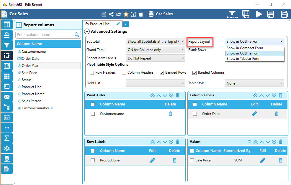
•The Report Layout can also be edited in the pivot table. Click the down arrow from the Report Layout to display choices.

•Select the desired layout by clicking on the desired choice.
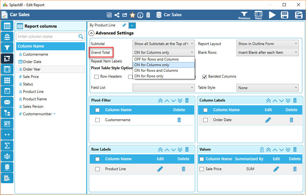
• Grand totals can be used for pivot table values by clicking the down arrow from this field.

• To add or remove grand totals for the data value, click the desired choice from the list.
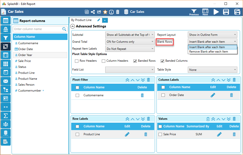
• Within the pivot table, users can separate each group of row data by using the inserting method to separate each change. The user can click the down arrow from the Blank Rows field to insert a blank after each item or remove a blank after each column.

Pivot Table Style Options:
For pivot table style options, users can have banned Rows, Banned Columns, Column Headers, or Row Headers.
•Banned Rows - This is a common term used in the United States in excel pivot functionality to group together rows. When a user chooses banned rows every row in the pivot table data will have a shade color.
•Banned Columns - This is a common term used in the United States in excel pivot functionality to group together columns. When a user chooses banned columns every column in the pivot table data will have a shade color.

Field List:
The field list is the column names of a data source a user can add to the pivot table by using the check mark choice next to the column name of information to bring in the pivot output or the drop and drag method. The list can be sorted for easy viewing for adding information to the pivot table.
•Click the down arrow from the field list box to reveal choices, select by clicking the desired sorting method.
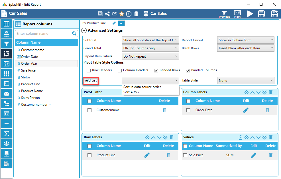
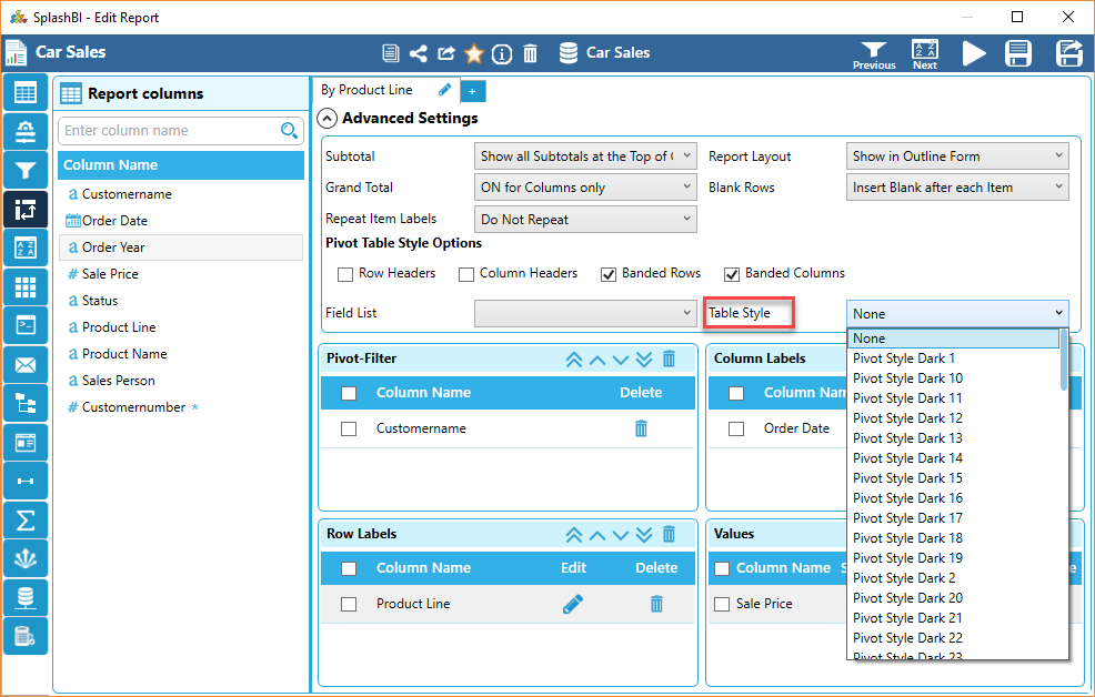
Table Style:
Within the excel pivot table options is a choice for table style. The table style ranges from dark to light with a variety of color intensity, this can be chosen from the creation of the pivot, or once the report has been downloaded into an excel output.
•Click the down arrow from the Table Style field to reveal color intensity choices.

Once all choices have been selected, click the arrow button![]() to exit from advanced settings.
to exit from advanced settings.
Once the user has finished the changes in Report Pivots, click 'Next' to proceed to the next screen.
To continue this tutorial, click here